Time Series Forecasting

Time Series Forecasting

Machine Learning

ARIMA (AutoRegressive Integrated Moving Average)

Perform d-th order differencing on the original sequence
Mathematically: $y^{(d)}_t = \Delta^d x_t$
- For $d=1$: $y_t = x_t - x_{t-1}$
- For $d=2$: $y_t = (x_t - x_{t-1}) - (x_{t-1} - x_{t-2})$
Fit an ARMA(p, q) model to the differenced sequence
\[y^{(d)}_t = \sum_{i=1}^{p} \phi_i y^{(d)}_{t-i} + \sum_{j=1}^{q} \theta_j \varepsilon_{t-j} + \varepsilon_t\]
- $\phi_i$ : AR (AutoRegressive) parameters
- $\theta_j$ : MA (Moving Average) parameters
- $\varepsilon_t$ : residuals
Rearranging the formula gives: $\varepsilon_t = y^{(d)}_t - \left(\sum_{i=1}^{p} \phi_i y^{(d)}_{t-i} + \sum_{j=1}^{q} \theta_j \varepsilon_{t-j}\right)$

We can compute all $\varepsilon_t$ by iterating over the sequence.
Construct the likelihood using Gaussian noise and compute the negative log-likelihood
Assume:
\[\varepsilon_t \sim \mathcal{N}(0,\, \sigma^2)\]
The log-likelihood for a single time step $t$ is:
\[\log p(\varepsilon_t) = -\frac{1}{2} \left( \frac{\varepsilon_t^2}{\sigma^2} + \log(2\pi\sigma^2) \right)\]
Set $\phi_i, \theta_j, \sigma$ as parameters, and optimize $\log p(\varepsilon_t)$.

Note: Fitting the noise in this way is equivalent to Maximum Likelihood Estimation (MLE)

时间序列模型(四)：ARIMA模型

chatgpt_arima

XGBoost

XGBoost: A Scalable Tree Boosting System

KDD 2016 Cited 68032

超详细解析XGBoost（你想要的都有）

Prophet

Formula: It is based on additive model:
\[y(t) = g(t) + s(t) + h(t) + \varepsilon_t\]
Where:

$g(t)$ — Trend

$s(t)$ — Seasonality (yearly / weekly / daily, etc.)

$h(t)$ — Holiday effects

$\varepsilon_t$ — Noise

Each component can be modeled using different methods.
Data It is a local model, built on a single time series.

The inputs include only the timestamps and the corresponding time series.

It can be seen as performing a series of feature engineering steps on the time variable: transform the time into various representations, transpose the data so that each timestamp becomes a row, and treat the time-based transformations as features.

Then it applies Lasso or Ridge regression for modeling.
\[X_t = [t, t^2, \sin(2 \pi t / 365), \cos( 2 \pi t /365), 1_{holiday}, ....]\] \[y_t = \text{observed value at time t}\]

chatgpt_propht

Deep Learning

TCN

An Empirical Evaluation of Generic Convolutional and Recurrent Networks for Sequence Modeling

arXiv 2018 Cited by 7490 TCN

N-BEATS

N-BEATS: Neural basis expansion analysis for interpretable time series forecasting

ICLR 2019 Cited by 1691

pytorch-forecasting

N-BEATS

NHITS

NHITS: Neural Hierarchical Interpolation for Time Series Forecasting

AAAI 2023 Cited by 621

TimesNet

TimesNet: Temporal 2D-Variation Modeling for General Time Series Analysis

ICLR 2023 Cited by 1529

RNN-based

LSTM

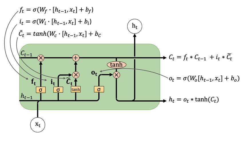
Overall, LSTM has three gates: the forget gate f, the input (memory) gate i, and the output gate o, corresponding respectively to c, [x, h], along with the new c (the new cell state is obtained by combining the previous two).

The cell state c stores long-term information, h is essentially the previous output, and x is the current input.
LSTM input shape: [batch_size, seq_len, feature_num]

LSTM output shape: [batch_size, seq_len, out_dim]

Hidden state h: [1, batch_size, out_dim]

Cell state c: [1, batch_size, out_dim]
It’s not broadcasting; it’s a loop. An LSTM is internally implemented as a loop that processes each time step individually. It splits the input along the second dimension so that each position’s time-step x is handled separately. At every time step, the LSTM module operations are performed, producing h and c for the next step.

❗️PyTorch’s LSTM hides this looping mechanism.
nn.LSTM specifies the input dimension and the hidden dimension. The final output includes only the hidden state h and cell state c from the last time step. Therefore, the hidden dimension and output dimension match.

Even though intermediate steps temporarily increase dimensionality when concatenating h and x, the weight matrices always project it back into the hidden dimension.
The final output is essentially all the h values concatenated along the second dimension.

LSTM

人人都能看懂的LSTM

Seq2seq

Sequence to sequence learning with neural networks

NeurIPS 2014 Cited by 28288

MQRNN

A Multi-Horizon Quantile Recurrent Forecaster

NeurIPS 2017 Cited by 608

LSTNet

Modeling Long- and Short-Term Temporal Patterns with Deep Neural Networks

SIGIR 2018 Cited by 2573

LSTNet

DeepAR (Deep Autoregressive)

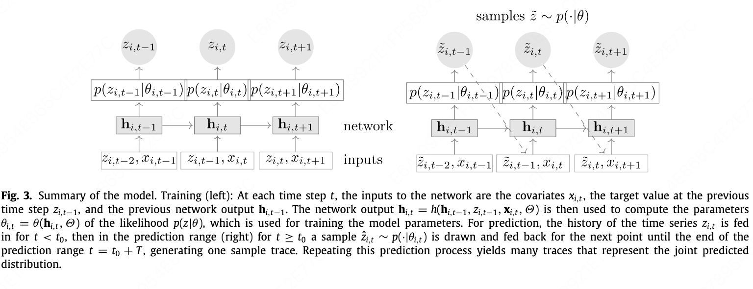
Using an LSTM as the basic module, with initial $c$ and $h$ set to 0. The input contains covariates $x$ and the previous step’s $z$ and $h$.
The model’s final outputs are $μ$ and $σ$, which are the two parameters of the distribution rather than the actual prediction value. The actual prediction must be obtained by sampling from the distribution defined by $μ$ and $σ$.
\[\begin{aligned} p_G(z \mid \mu, \sigma) &= (2 \pi \sigma^2)^{-1/2} \exp (-(z - \mu)^2 / (2 \sigma^2)), \\ \mu(h_{i,t}) &= w_{\mu}^T h_{i,t} + b_{\mu}, \\ \sigma(h_{i,t}) &= \log (1 + \exp(w_{\sigma}^T h_{i,t} +b_{\sigma})) \end{aligned}\]
The model is trained using the log-likelihood as the loss function. The $p$ corresponds to the distribution determined by $μ$ and $σ$, and $z$ is the ground truth.
\[L = \sum_{i=1}^N \sum_{t=t_0}^{T} \log p(z_{i,t} \mid \theta (h_i,t))\]
In essence, prediction involves sampling from the distribution, while training uses the true value to compute the likelihood and infer the distribution parameters. During training, each time step of every sequence outputs a $μ$ and $σ$, and prediction works the same way.
During training, the model uses the true $z_{i,t-1}$ to predict $z_{i,t}$. However, during inference it uses the previously predicted $z_{i,t-1}$. The paper acknowledges this issue but claims it does not observe an impact. Still, this is clearly questionable. In the terminology of lstm_linear, this is essentially an IMS (Iterated Multi-Step) model

DeepAR

DeepAR: Probabilistic forecasting with autoregressive recurrent networks

International Journal of Forecasting 2020 Cited by 2524

pytorch-forecasting

DeepAR-pytorch

Transformer-based

LogTrans/Time-Series Transformer

Enhancing the Locality and Breaking the Memory Bottleneck of Transformer on Time Series Forecasting

NeurIPS 2019 Cited by 2045

Longformer

Longformer: The Long-Document Transformer

arXiv 2020 Cited by 4690

Reformer

Reformer: The Efficient Transformer

ICLR 2020 Cited by 3152

Informer

The paper proposes an improved variant of the original Transformer model, with three main modifications:

ProbSparse Attention: By comparing the attention distribution with a uniform distribution, the model reduces the time and space complexity of the attention mechanism from $O(L^2)$ to $O(L \ln L)$, where $L$ is the sequence length.
Self-attention Distillation: By inserting max-pooling layers between attention modules, the model further reduces memory usage.
Generative Inference: Instead of autoregressively generating predictions one token at a time, the model directly predicts the entire sequence in one step.

The final model outperforms LSTM, Reformer, and several other baselines.

Informer: Beyond Efficient Transformer for Long Sequence Time-Series Forecasting

AAAI 2021 Cited by 4838

Informer2020

Autoformer

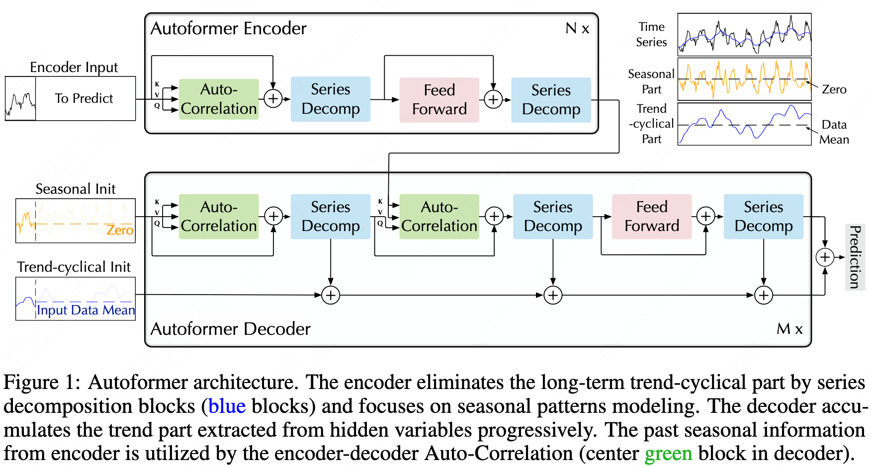
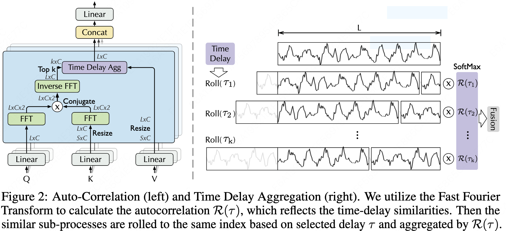
Auto-correlation: The attention mechanism is applied After the sliding operation and Fourier decomposition in frequency domain. Only the top $logL$ sliding attention scores are selected. $$ \begin{aligned} S_{xx}(f) &= F(X_t) F^*(X_t) = \int_{-\infty}^{\infty} X_t e^{-i 2 \pi t f} dt \overline{\int_{-\infty}^{\infty} X_t e^{-i 2 \pi t f} dt} \

R_{xx}(\tau) &= F^{-1}(S_{xx}(f)) = \int_{-\infty} {\infty} S_{xx}(f) e^{i 2 \pi f \tau} df \end{aligned} $$
\[\tau_1, ..., \tau_k = \arg_{\tau \in (1, ..., L)} \text {Topk} (R_{Q,K}(\tau)) \\ \hat{R}_{Q,K}(\tau_1), ..., \hat{R}_{Q,K}(\tau_k) = \text {SoftMax} (R_{Q,K} (\tau_1), ..., R_{Q,K} (\tau_k)) \\ \text{Auto-Correlation}(Q,K,V) = \sum_{i=1}^k \text{Roll} (V, \tau_i) \hat{R}_{Q,K} (\tau_i)\]
Serires decomposition:
\[X_t = \text{Avgpool(\text{Padding(X)})} \\ X_s = X - X_t\]
Input The encoder input is vector of sequence length.

The decoder input is vector of label length plus some zeros, or the average of the input part.
Positional encoding

Transformer中Position Embedding的原理与思考

Cannot distinguish the order of relations?

Transformer学习笔记一：Positional Encoding（位置编码）
Token Embedding A 1D convolution is used instead of a linear layer.

This captures the relationships between adjacent time points, which is equivalent to applying convolution kernels along the time dimension (the second-to-last dimension), while transforming the feature dimension (the last dimension) to the d_model dimension.

This step is essentially a CNN.

Convolution layer parameter count: The parameter count for each convolution kernel is the kernel size multiplied by the number of input channels. The number of convolution kernels equals the number of output channels. (Clearly, different convolution kernels for different channels should be used.)

If bias is considered, then an additional vector of the length equal to the number of output channels is added.

Fully connected layer parameter count is the size of the weight matrix, which is the number of input channels multiplied by the number of output channels.

If bias is considered, an additional vector of length equal to the number of output channels is added.

In this scenario, the convolution is equivalent to each feature channel multiplying and summing with the convolution kernel, and the final sum results in a value. There are d_model such convolution kernels.

This process first integrates features across local time dimensions at the feature level, then adds across features, finally generating internal features in multiple dimensions.

This seems quite reasonable.
Additionally, there is a Temporal Embedding.

Positional encoding using sine and cosine functions on the monthly, weekly, daily, and minute dimensions.

Each dimension is assigned a specific sequence length, and these are summed together. This is impressive!

The source code seems to set different sequence lengths based on the dataset, which should be modified. Originally, it assumed data was gathered every 15 minutes.
FFT The complexity of formulas 6 and 7 is $O(L \log L)$ because the top $L \log L$ sequences are selected, whereas formula 5 is not, and it has $O(L^2)$. By using the FFT in formula 8, with its recursive properties, it can achieve $O(L \log L)$.

The FFT result is used as a weight to multiply the input sequence, rolling the corresponding time intervals of the sequence.

This is equivalent to transforming the previous input to get the output?

It still seems to go against the original purpose of the Transformer. It’s like blending words that can only appear in the same sentence as previous words?

The FFT here is applied only to the sequence dimension, while the process for each feature dimension is completely independent.

Multi-head attention in the Auto-correlation part is actually exactly the same; only the FeedForward layer right after has feature interactions between layers.

Autoformer_1 Autoformer_2

Autoformer: Decomposition Transformers with Auto-Correlation for Long-Term Series Forecasting

NeurIPS 2021 Cited by 2438

TFT (Temporal Fusion Transformers)

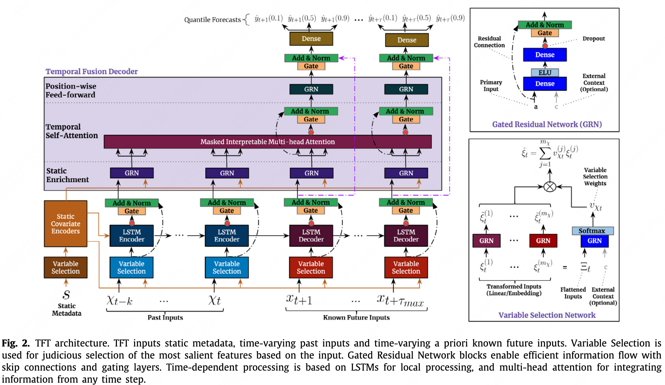
It is compared with the LogTrans, DeepAR and MQRNN. It is an attention-based DNN architecture and is almost unrelated to the classical Transformer in terms of structure.
In terms of data structure, the model considers that many variables are not known at prediction time, such as historical customer traffic.
The input contains four parts:

Static Covariates, $s_i$, static_reals and static_categoricals in pytorch-forecasting

Observed/Unknown Inputs, $z_{i,t-k:t}$, time_varying_unknown_reals and time_varying_unknown_categoricals in pytorch-forecasting

Known Inputs, $x_{i,t-k:t+\tau}$, time_varying_known_reals and time_varying_known_categoricals in pytorch-forecasting

Target till the start time, $y_{i,t-k:t}$

$s_i$ is input into the Variable Selection, as the ‘Static Metadata’. $z_{i,t-k:t}$, $x_{i,t-k:t}$, $y_{i,t-k:t}$ are input into the encoder part, as the ‘Past inputs’. $x_{i,t:t+\tau}$ is input into the decoder part, as the ‘Known Future Inputs’. Both for training and testing.
Layer Norm
Gating mechanism: to introduce nonlinear relationships only where needed. $GRN_w(a,c) = \text{LayerNorm} (a + GLU_w ( \eta_1)) \\ \eta_1 = W_{1,w} \eta_2 + b_{1,w} \\ \eta_2 = ELU(W_{2,w} a + W_{3,w} c + b_{2,w}) \\ GLU_w(\gamma) = \sigma(W_4,w \gamma + b_{4,w}) \odot (W_{5,w} \gamma + b_{5,w})$
Variable selection: $v_{X_t} = Softmax(GRN_{v_X} (\Xi_t, c_s)) \\ \hat{\xi}_t^{(j)} = GRN_{\hat{\xi}(j)} (\xi_t^{(j)}) \\ \hat{\xi}_t = \sum_{j=1}^{m_X} v_{X_t}^{(j)} \hat{\xi}_t^{(j)}$

$\xi_t^{(j)}$, Embedded input of the jth variable at time t

$\Xi_t={[{\xi_t^{(1)}}^T, …, {\xi_t^{(m_x)}}^T]}^T$, the flattened vector of inputs at time t.

Input the embedded vector of every feature into the GRU seperately and input the concated vector at time t into the GRU and softmax, then muptiply and sum those two result, as a weighting process.
LSTM the same as the original one.
Interpretable Muti-head Attention: $\begin{aligned} \hat{H} &= \hat{A} \, (Q, \, K)V \, W_V \\ &= \left\{\frac{1}{m_H} \sum_{h=1}^{m_H} A (Q W_Q^{(h)}, K W_K^{(h)}) \right\} V W_V, \\ &= \frac{1}{m_H} \sum_{h=1}^{m_H} \text{Attention} (Q W_Q^{(h)}, K W_K^{(h)}, V W_V) \end{aligned}$
Quantile prediction
Loss function: $L(\Omega, W) = \sum_{y_t \in \Omega} \sum_{q \in Q} \sum_{\tau=1}^{\tau_{max}} \frac{QL(y_t, \hat{y} (q, t- \tau, \tau), q)}{M \tau_{max}} \\ QL(y, \hat{y}, q) = q ( y - \hat{y})_+ + (1 - q)(\hat{y} - y)_+$
Both PyTorch Forecasting and Kaggle did not properly separate the validation set.

Using the test set for Optuna hyperparameter tuning obviously leads to data leakage.

TFT

Temporal Fusion Transformers for interpretable multi-horizon time series forecasting

International Journal of Forecasting 2021 Cited by 1835

Demand forecasting with the Temporal Fusion Transformer

【时序】TFT：Temporal Fusion Transformers

Pytorch Forecasting => TemporalFusionTransformer

Store Sales - Time Series Forecasting

Fedformer

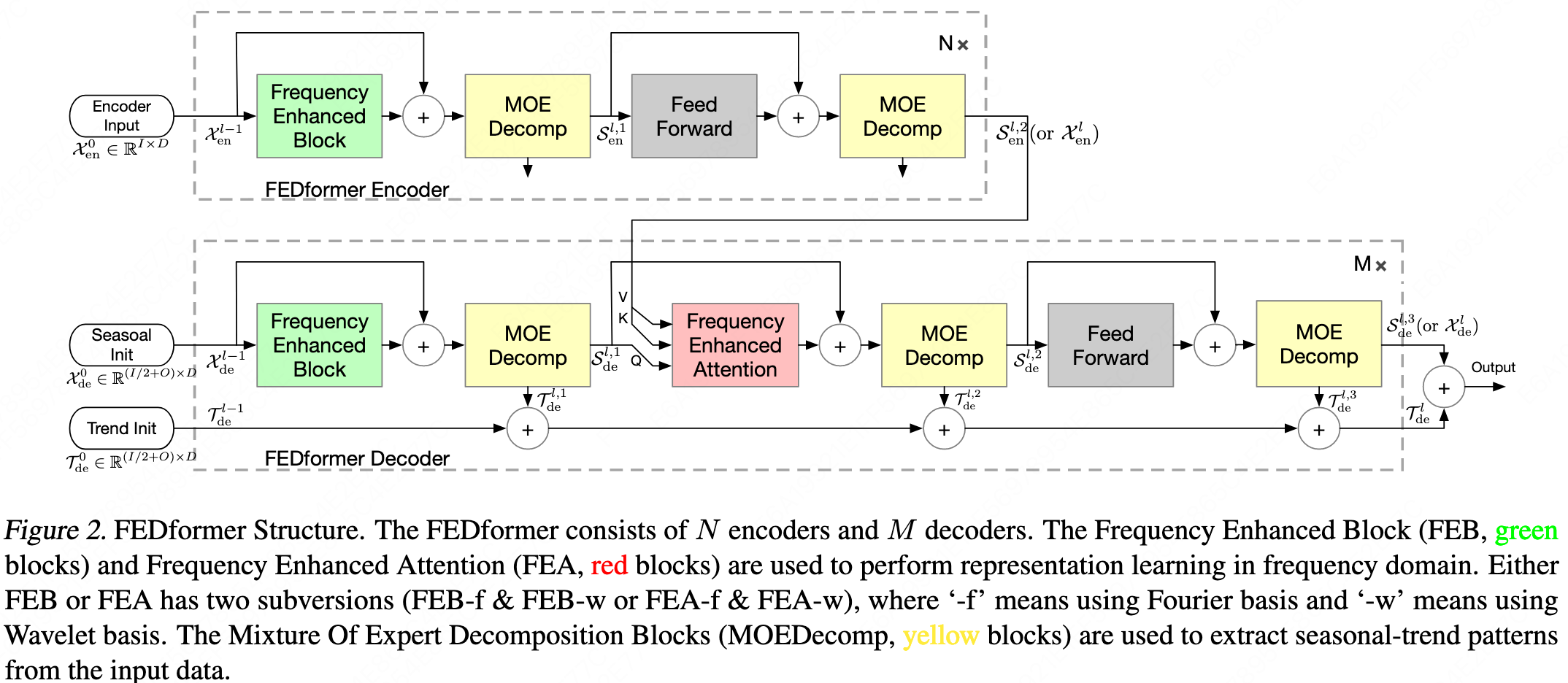
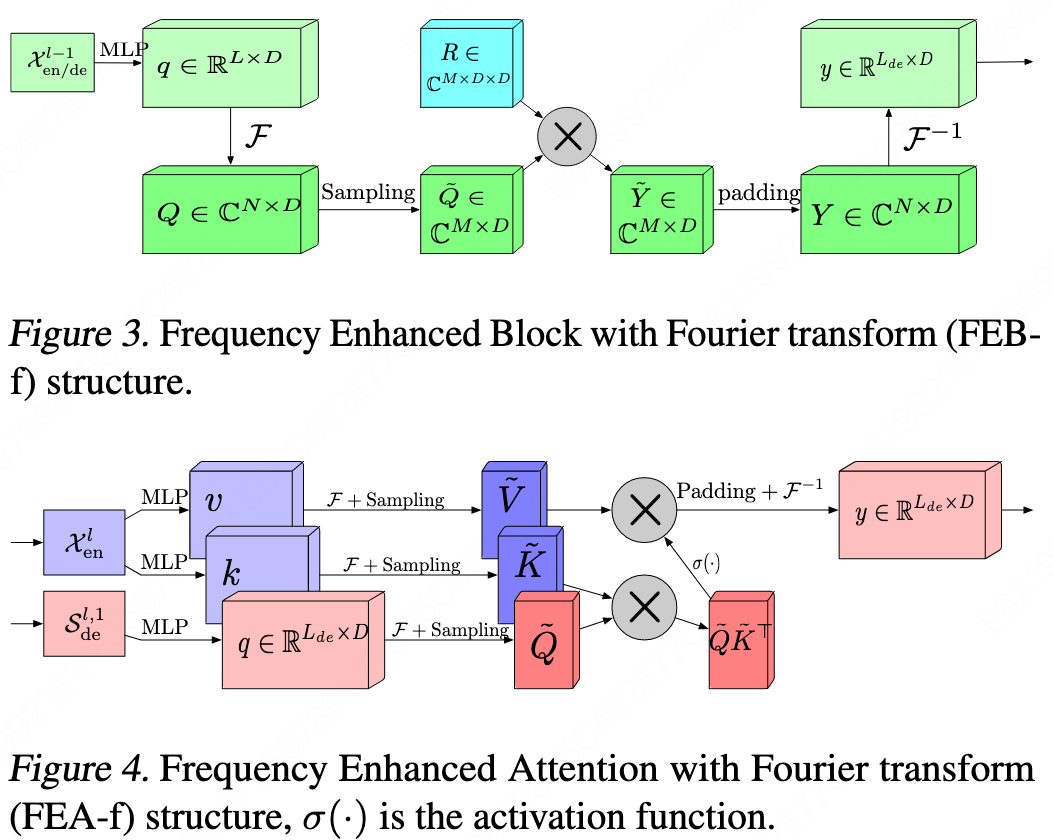
It can be considered an upgraded version of Autoformer. The overall architecture is consistent with Autoformer, but many details and sub-modules differ. The results are also compared directly against Autoformer.
Wavelet transform is added on top of the Fourier transform.
The top-k selection is replaced by random selection, and it is applied before the $q_k$ multiplication.
A MoE (Mixture of Experts) mechanism is added to the frequency-domain decomposition.
\[X_{trend} = Softmax(L(x)) * (F(x))\]
The related work section of this paper is extremely comprehensive and very well organized.

Fedformer_1 Fedformer_2

FEDformer: Frequency Enhanced Decomposed Transformer for Long-term Series Forecasting

PMLR 2022 Cited by 1960

ICML2022-FEDformer

Pyraformer

Pyraformer: Low-Complexity Pyramidal Attention for Long-Range Time Series Modeling and Forecasting

ICLR 2022 Cited by 934

PatchTST

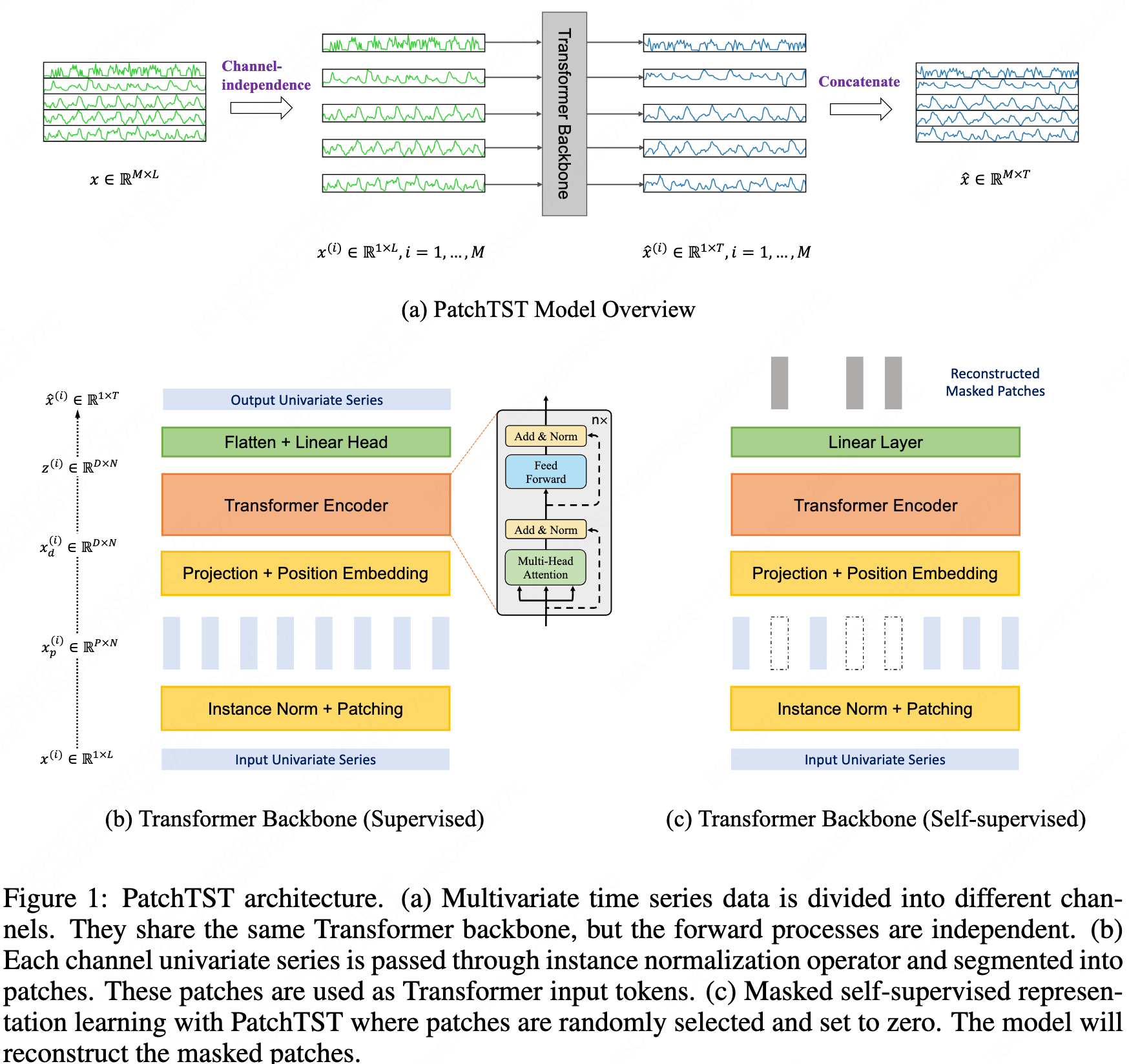
Patching

The sequence is truncated into patches and then transposed so that each patch becomes a single token.
Channel independence

Each variable’s time series is fed into the Transformer independently, without interacting with other variables.
Normalization

This is instance normalization, which is fine — it does not mix information across different features.
Linear layer

A single weight matrix is applied to all (batch_size, n_variables, patch_num), transforming the dimension from patch_len to d_model.

Although instance normalization is applied, giving each feature the same influence is clearly unreasonable, and there is no interaction between features.

Therefore, this should not be considered a linear layer but rather an embedding layer.
Attention layer

Positional encoding addition: PyTorch’s broadcasting mechanism aligns dimensions from right to left when adding positional encodings.

Encoder input: batch_size and n_vars are merged into a single dimension before being passed into the encoder, which is consistent with the channel-independent design.

Multi-head attention: The view operation reorganizes dimensions from right to left, splitting the last dimension first.

QK multiplication: matmul multiplies the last two dimensions; d_k disappears as the inner dimension.

The resulting attention weights/scores have shape (q_len, q_len).

Thus, different features are treated equally.The attention weights represent the correlations between patches at different positions, and there are linear layers with d_model dimensions both before and after.

PatchTST

A Time Series is Worth 64 Words: Long-term Forecasting with Transformers

ICLR 2023 Cited by 1390

PatchTST

Crossformer

Crossformer: Transformer Utilizing Cross-Dimension Dependency for Multivariate Time Series Forecasting

ICLR 2023 Cited by 937

iTransformer

Inverted: Embedding the whole series as the token.
It is a framework and a bundle of efficient attention mechanisms can be the plugins.

iTransformer

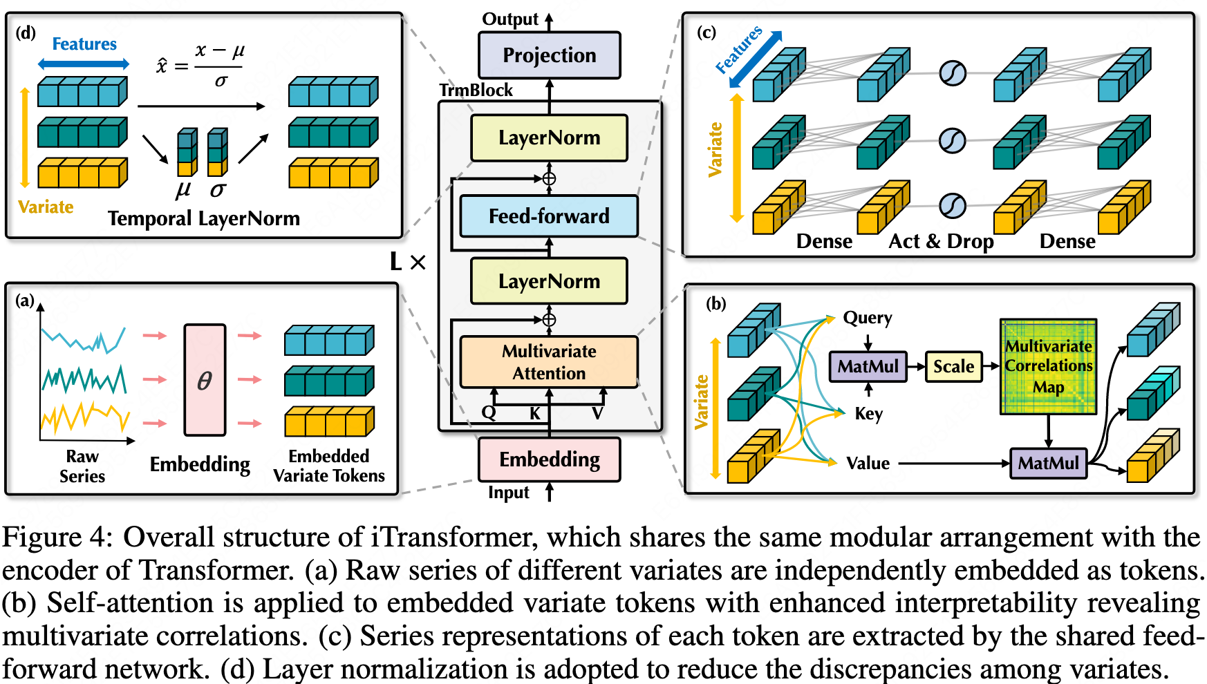
iTransformer: Inverted Transformers Are Effective for Time Series Forecasting

ICLR 2024 Cited by 659

iTransformer

PDF

Periodicity Decoupling Framework for Long-term Series Forecasting

ICLR 2024 Cited by 35

PDF

DUET

DUET: Dual Clustering Enhanced Multivariate Time Series Forecasting

KDD 2025 Cited by 8

Duet

LLMs-based

One fits all

OneFitsAll

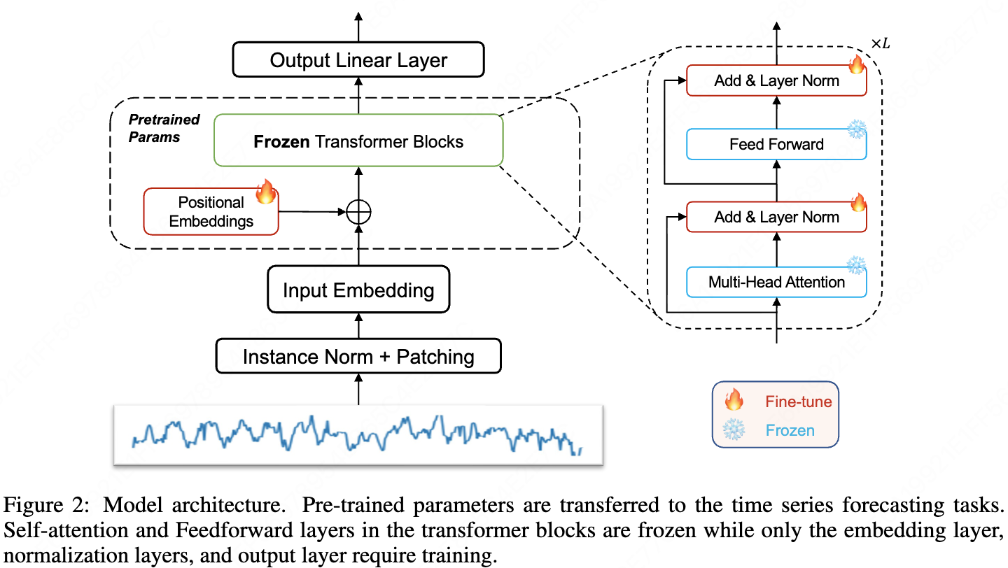
Fine-tune the positional embedding and layer normalization of the backbone LLM model. Also Add a input embedding, a output Linear layer and a instance normalization plus patching.
The same patch method as patchTST.
Isn’t fine-tuning require large scale dataset?
Few-shot is using the first 5%/10% time steps as the new base dataset and the input and the label arrays would be taken from it by sliding. This proccess only affects the training set.
Zero-shot means examining how well a model performs on a dataset♣ when it is optimized on another dataset.
The dataset in few-shot and zero-shot is different?

One Fits All: Power General Time Series Analysis by Pretrained LM

NeurIPS 2023 Cited by 508

NeurIPS2023-One-Fits-All

TimeGPT

TimeGPT-1
arXiv 2023 Cited by 289

Nixtla / TimeGPT

TimesFM

ICML 2024 Cited by 392

Google Research / TimesFM

Chronos

arXiv 2024 Cited by 417

Amazon Science / Chronos

Time-LLM

TIMELLM

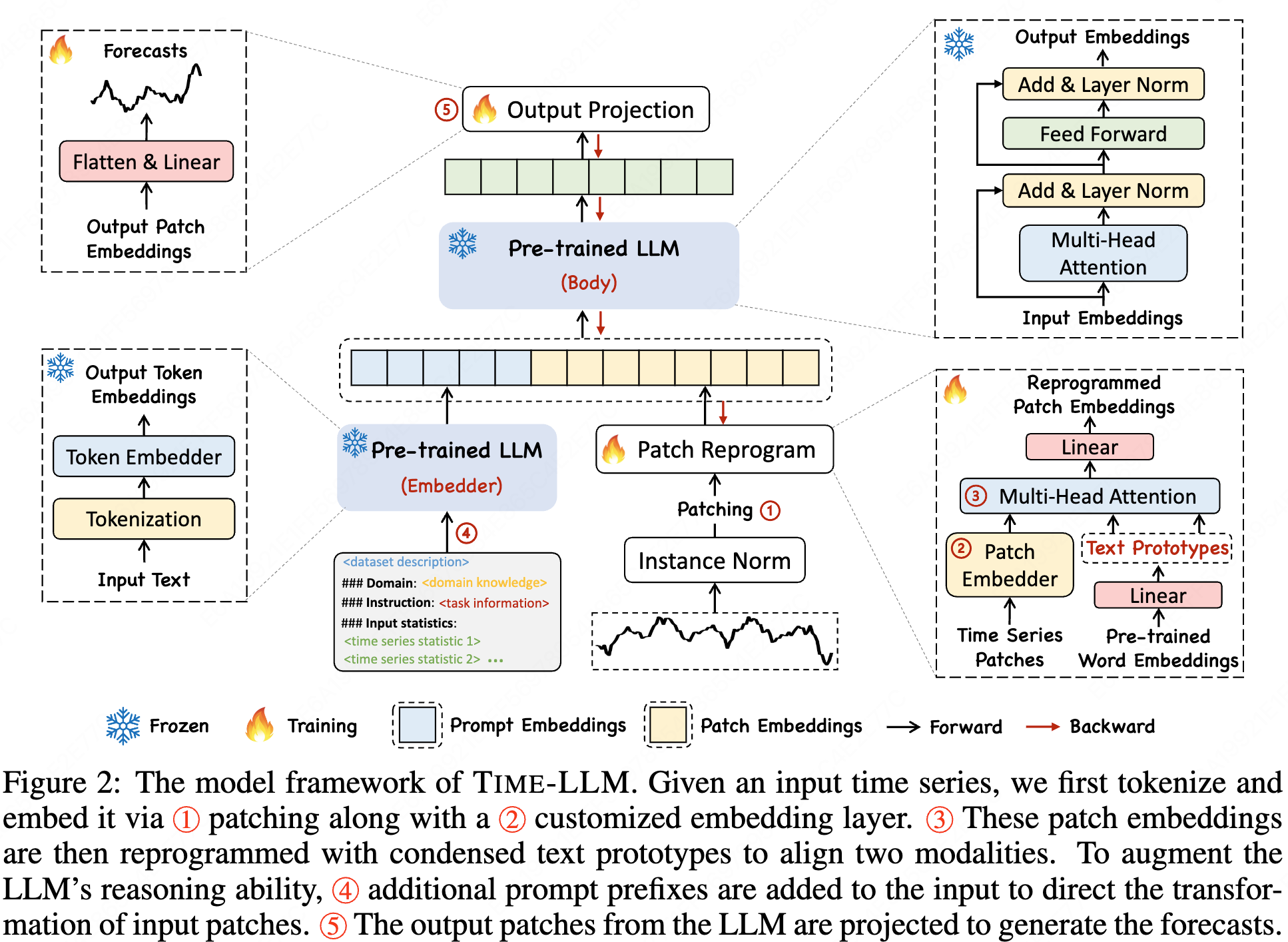
A reprogramming framework to adapt LLMs for time series forecasting while keeping the backbone moder intact.
The OneFitsAll framework still uses fine-tuning while this work remaining the LLM weight unchanged.
The same patch method as patchTST.
Reprogramming is not simply linear embedding because ‘time series can neither be directly edited nor described losslessly in natural language.’ It first embeds patches and use linear layer to combine word embeddings (the embeddings of the backbone LLM) at the same time. Then use a attention layer to process the embedded patches and combined word embeddings (prototypes). It is a Encoder-Decoder attention layer in original transformer with patches as the query and prototypes as the key and value. It is similar to a translation proccess.
Output just projects the natural language back to time series data.
The defination of few-shot is the same as One Fits All. But there is no code for few-shot and zero-shot training and testing?
The figure 5 is likely to be the weight of the attention layer and the linear layer generating prototypes.

Time-LLM

ICLR 2024 Cited by 797

KimMeen / Time-LLM

CALF

AAAI 2025 Cited by 21

LLM4TS

TIST 2025 Cited by 158

blacksnail789521 / LLM4TS

Leadboard

TFB

TFB: Towards Comprehensive and Fair Benchmarking of Time Series Forecasting Methods

PVLDB 2024 Cited by 46

decisionintelligence / TFB

Time-Series-Library

thuml / Time-Series-Library

Review

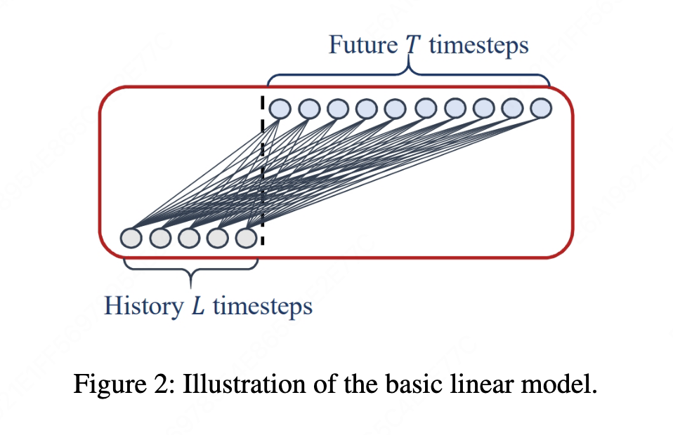
LTSF-Linear

Linear layers are channel-independent

It maps the input sequence length to the output sequence length instead of mapping input channels to output channels.

linear_model

DLinear and NLinear feel like they are imitating ARIMA, and they’re even less sophisticated—after all, the former two don’t combine their components the way ARIMA does. So why were earlier models stronger than ARIMA, yet weaker than these two models? Is it because of the difference between DMS and IMS?
For exchange-rate time-series forecasting, machine learning performs worse than simply repeating the last value. This suggests that, to some extent, predicting exchange rates from historical data is not very meaningful—machine-learning models just overfit. Conceptually, this might be because exchange rates are the result of strategic interactions (a game-theoretic equilibrium).
This “qualitative result” figure makes it look like the authors didn’t train those transformer networks properly.
Indeed, almost every previous paper mentions that the scenario is LTSF, which probably aligns with the fact that transformers were originally designed to deal with the vanishing-gradient problem of RNNs and to learn long sequences.
We definitely need to include cabinet or store identifiers; something channel-independent like Linear would absolutely be wrong❗️

The linear layer in NLinear operates on the temporal dimension, while the channel dimension effectively stays in a fixed order.

But the issue is that here the “channels” are equivalent to the batch dimension, so everything gets averaged as if they were the same sample.

So we can only say the data are independent, but the processing is completely identical—it’s all using the same weight matrix.

Are Transformers Effective for Time Series Forecasting?

AAAI 2023 Cited by 2310

LTSF-Linear

LLMsForTimeSeries

NeurIPS 2024 Cited by 84

BennyTMT / LLMsForTimeSeries

Bergmeir NeurIPS Talk

“Qiu et al. (PVLDB, 2024): PatchTST evaluates using a ‘Drop Last trick’”, the mentioned paper corresponds to the TFB paper.
It presents solid criticisms of many Transformer- and LLM-based time-series forecasting papers, and reaffirms the value of traditional models such as N-BEATS and DHR-ARIMA. It also recommends several newly released models, such as Chronos, TimeGPT, and TimesFM, but it’s unclear what distinguishes these recommended new models from one another.
Regarding datasets, it basically recommends only M4 and Monash, while raising concerns about the others.
This is especially true for economics-related datasets such as stock prices and exchange rates, since markets tend to be efficient and offer no exploitable additional information for forecasting. For weather-related datasets such as electricity demand, experts generally believe forecasting more than two weeks ahead is unrealistic.
It even questions the very existence or justification of global models / foundation models (where the dataset contains multiple time series; local models use only a single series). If many unrelated features are all used together as part of the loss function, they can negatively impact the model’s performance on the target domain/features. ❗️
Corresponding to the ambiguity of language models, time-series models also need clarification. But the problem is: humans themselves might not know these clarifications. Are we supposed to turn time-series models into something like a chatbot that experts can interact with, continuously supplying contextual information? ❓

Fundamental limitations of foundational forecasting models: The need for multimodality and rigorous evaluation

Transformers for TSF

A Closer Look at Transformers for Time Series Forecasting: Understanding Why They Work and Where They Struggle

ICML 2025 Cited by 0

Dataset

Multivariate Time series Data sets

All the datasets used by the Transformer-based models above come from this library.

laiguokun / multivariate-time-series-data

Monash

Monash Time Series Forecasting Archive

arXiv 2021 Cited by 259

Monash Time Series Forecasting Repository

laiguokun / multivariate-time-series-data

M4

Each CSV file contains data with a different time granularity.
Each row is a time series, and the length of each time series may vary.
Each column is just a placeholder and does not imply that the same column corresponds to the same time step.

The M4 Competition: 100,000 time series and 61 forecasting methods

arXiv 2021 Cited by 259

M4 Forecasting Competition Dataset

Makridakis Competitions

Mcompetitions / M4-methods

M5

M5 Forecasting - Accuracy

M6

The M6 forecasting competition: Bridging the gap between forecasting and investment decisions